Higher Order Linear Regression

Challenge :

The goal of this assignment is to learn about the concept of overfitting using the Higher order linear regression.

Also we are going to create a polynomial model with degrees 0,1,3,9 and compare the performances of all the degrees.

Note : Used references are highlighted with number in green color

---

What is Linear Regression? [1]

Linear Regression is a machine learning algorithm based on supervised learning. It performs a regression task. Regression models a target prediction value based on independent variables. It is mostly used for finding out the relationship between variables and forecasting.

Linear regression performs the task to predict a dependent variable value (y) based on a given independent variable (x). So, this regression technique finds out a linear relationship between x (input) and y(output). Hence, the name is Linear Regression.

In the figure below, X (input) is the work experience and Y (output) is the salary of a person. The regression line is the best fit line for our model.

---

1. Generating data pairs:

We will generate 20 data pairs using y = sin(2*pi*X) + 0.1 * N and divide them equally into train and test data set. Use uniform distribution between 0 and 1 for X . Use sample N from the normal gaussian distribution.

X = np.random.uniform(0, 1, 20)
X = np.array([[i] for i in X])
N = np.random.normal(0,1,20)
Y = []
for x,n in zip(X,N):
	y = np.sin(2 * np.pi * x) + 0.1 * n
	Y.append(list(y)[0])
	
Y = np.array(Y)
train = {'x': X[:10], 'y': Y[:10]}
test = {'x':X[10:], 'y':Y[10:]}

2. Find weights of polynomial regression:

we are going to find weights of polynomial regression order using gradient descent algorithm minimizing the error for order 0,1,3,9.

3. Display weights in table:

After performing the gradient descent algorithm with iterations of 500 using learning rate0.01 we obtained

the below weights displayed in the table.

0	1	3	9
-0.33362086	-0.33362086	-0.33362086	-0.33362086
	-0.38081357	-0.25176075	-0.21833381
		-0.12844771	-0.21357692
		0.01012239	-0.16120512
			-0.09524989
			-0.02991933
			0.03014103
			0.08361317
			0.13043797
			0.17107172

4. Draw a chart of fit data:

In this, we’re taking all the weights w and creating the polynomials to plot against our training data. We are going to see how well each polynomial looks with respect to the training data

The below graphs are obtained with learning rate of 0.01 and iterations of 500 on gradient descent algorithm..

def main(train, test, degrees, learning_rate, iterations) :
    
	for deg in degrees:
		model = PolynomailRegression( degree = deg, learning_rate = learning_rate, iterations = iterations )
		pp.append(model.fit( train['x'], train['y'] )[1])
		Y_pred = model.predict( test['x'] )
		Y_pred_train = model.predict(train['x'])
		test_rmse.append(mean_squared_error(test['y'], Y_pred, squared=False))
		train_rmse.append(mean_squared_error(train['y'], Y_pred_train, squared=False))
	
		plt.scatter( test['x'], test['y'], color = 'blue' )
	
		plt.plot( test['x'], Y_pred, color = 'orange' )
	
		plt.title( 'X vs Y for ' +str(deg) )
	
		plt.xlabel( 'X' )
	
		plt.ylabel( 'Y' )
	
		plt.show()

Graphs for order 0 and 1

Graphs for order 3 and 9

5. Draw train error vs test error :

The below graph interprets the train and test root mean square error against test and train data.

6. Now generate 100 more data and fit 9th order model and draw fit:

Here again we are going to generate 100 more points for the same 9th order model instead of earlier used 20 points and drawing a fit for that. The below mentioned is the graph of the model.

7. Now we will regularize using the sum of weights: [2]

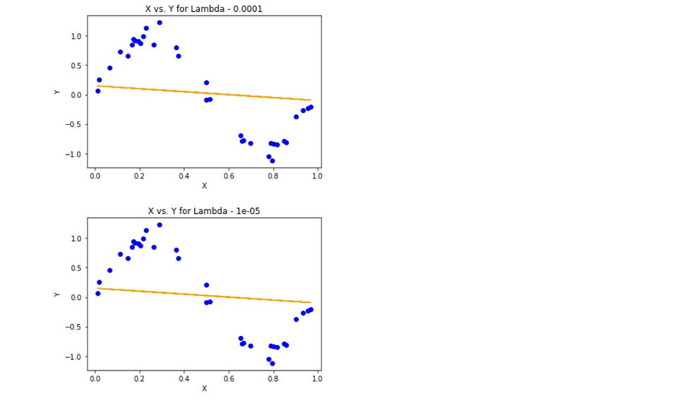
Regression with L2 regularization is also known as ridge regression, The following is the graph for the various values of lambda with 100 iterations of the gradient descent algorithm and learning rate of 0.01.

8.Charts for lambda is 1, 1/10, 1/100, 1/1000, 1/10000, 1/100000:

9. Now draw test and train error according to lamda:

The below graph illustrates the Root Mean squared error over on various values of lambda as mentioned

Jupyter Notebook [3]

Notebook

My Contribution

So by using the mentioned references I have hyper parameter tuned the Higher order regression. by changing the number of iterations, learning rate and lambda values for minimizing the error.

Form the above graphs we can see that the Regression with Regularization has performed more accurately than the Higher order linear regression. As Regularization helps in reducing the noise in the data. The Error of Regression with regularization on test data is less than the higher order regression.

Challenges and how i solved them

It was difficult to implement without using the libraries for the regression with regularization. So used some of the mentioned references to implement sum of weights

with regulariza0tion. and To get more accuracy i have tuned the Higher order regression. by changing the number of iterations, learning rate and lambda values for minimizing the error.

Overfitting and Underfitting [4]

Overfitting:

A statistical model is said to be overfitted when we train it with a lot of data (just like fitting ourselves in oversized pants!). When a model gets trained with so much data, it starts learning from the noise and inaccurate data entries in our data set. Then the model does not categorize the data correctly, because of too many details and noise. The causes of overfitting are the non-parametric and non-linear methods because these types of machine learning algorithms have more freedom in building the model based on the dataset and therefore they can really build unrealistic models. A solution to avoid overfitting is using a linear algorithm if we have linear data or using the parameters like the maximal depth if we are using decision trees.

Underfitting: A statistical model or a machine learning algorithm is said to have underfitting when it cannot capture the underlying trend of the data. (It’s just like trying to fit undersized pants!) Underfitting destroys the accuracy of our machine learning model. Its occurrence simply means that our model or the algorithm does not fit the data well enough. It usually happens when we have fewer data to build an accurate model and also when we try to build a linear model with fewer non-linear data. In such cases, the rules of the machine learning model are too easy and flexible to be applied on such minimal data and therefore the model will probably make a lot of wrong predictions. Underfitting can be avoided by using more data and also reducing the features by feature selection.